
221 Episodes · 77h15min
- Split Pane Animations (Part 2) 14:21
- Split Pane Animations (Part 1) 12:44
- Swift, the Language: The FormatStyle API 22:32
- The Layout Protocol (Part 4) 19:40
- The Layout Protocol (Part 3) 16:51
- The Layout Protocol (Part 2) 25:19
- The Layout Protocol (Part 1) 28:30
- Matched Geometry and Corner Radius 28:30
- Interpolating Matched Geometry Effect 28:30
- Matched Geometry Effect for Positioning Badges 23:35
- Solving the View Model Problem (Part 3) 17:01
- Solving the View Model Problem (Part 2) 14:59
- Solving the View Model Problem (Part 1) 18:59
- Settings Form Layout (Part 2) 16:40
- Settings Form Layout (Part 1) 21:56
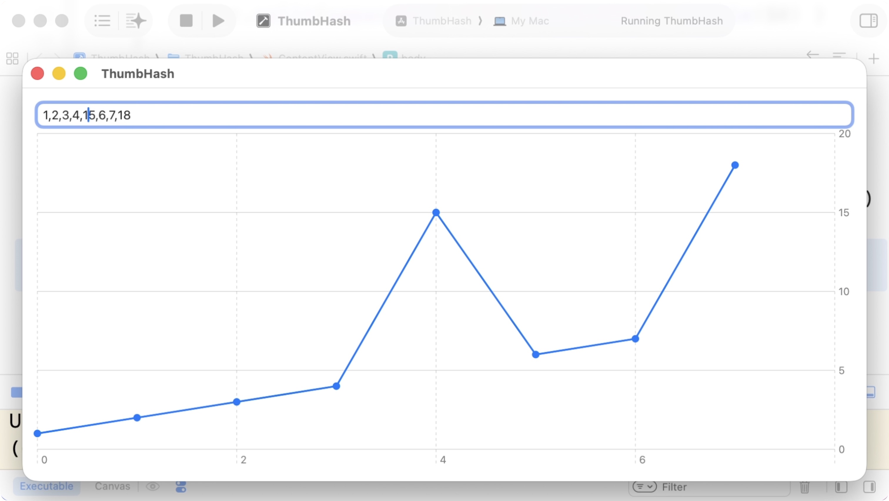
- ThumbHash (Part 6) 16:54
- ThumbHash (Part 5) 19:12
- ThumbHash (Part 4) 31:06
- ThumbHash (Part 3) 21:19
- ThumbHash (Part 2) 22:26
- ThumbHash (Part 1) 22:26
- Visual Node Editor (Part 9) 22:29
- Visual Node Editor (Part 8) 18:51
- Visual Node Editor (Part 7) 24:59
- Visual Node Editor (Part 6) 15:57
- Visual Node Editor (Part 5) 17:09
- Visual Node Editor (Part 4) 31:52
- Visual Node Editor (Part 3) 20:01
- Visual Node Editor (Part 2) 15:39
- Visual Node Editor (Part 1) 27:10
- SwiftUI as Static Site Generator (Part 6) 32:13
- SwiftUI as Static Site Generator (Part 5) 21:21
- SwiftUI as Static Site Generator (Part 4) 28:18
- SwiftUI as Static Site Generator (Part 3) 20:58
- SwiftUI as Static Site Generator (Part 2) 20:38
- SwiftUI as Static Site Generator (Part 1) 22:16
- Building a Token Field (Part 5) 27:40
- Building a Token Field (Part 4) 16:06
- Building a Token Field (Part 3) 19:05
- Building a Token Field (Part 2) 25:12
- Building a Token Field (Part 1) 23:10
- Building a FaceTime-like Animation (Part 2) 18:48
- Building a FaceTime-like Animation (Part 1) 16:08
- Staggered Animations Revisited (Part 3) 14:03
- Staggered Animations Revisited (Part 2) 16:31
- Staggered Animations Revisited 00:00
- Custom Format Styles 20:31
- Text Formatting 21:13
- Keeping Local View State in Sync 19:35
- Optional Bindings 27:15
- Attribute Graph (Part 10) 17:10
- Attribute Graph (Part 9) 32:16
- Attribute Graph (Part 8) 20:57
- Attribute Graph (Part 7) 23:53
- Attribute Graph (Part 6) 25:44
- Attribute Graph (Part 5) 28:20
- Attribute Graph (Part 4) 26:32
- Attribute Graph (Part 3) 20:10
- Attribute Graph (Part 2) 22:12
- Attribute Graph (Part 1) 20:35
- Particle Effects (Part 6) 15:02
- Particle Effects (Part 5) 12:37
- Particle Effects (Part 4) 21:04
- Particle Effects (Part 3) 18:16
- Particle Effects (Part 2) 16:25
- Particle Effects (Part 1) 14:28
- Lazy Container Views (Part 4) 28:54
- Lazy Container Views (Part 3) 20:16
- Lazy Container Views (Part 2) 18:50
- Lazy Container Views (Part 1) 16:05
- Bento Layout (Part 4) 10:06
- Bento Layout (Part 3) 27:25
- Bento Layout (Part 2) 13:33
- Bento Layout (Part 1) 13:16
- Environment & Preference Updates 15:30
- Tooltips (Part 2) 00:00
- Tooltips (Part 1) 17:14
- Detecting Visible Cells 17:57
- Debugging Animations 23:16
- Picker Animation (Part 2) 13:59
- Picker Animation (Part 1) 17:06
- Wobble Animation 21:08
- Positioning Badges (Part 2) 17:56
- Positioning Badges (Part 1) 14:10
- Reimplementing the Default Button Style 18:17
- Conditional Aspect Ratio Modifier (Part 2) 17:45
- Conditional Aspect Ratio Modifier (Part 1) 21:20
- Building a Legend View (Part 3) 18:22
- Building a Legend View (Part 2) 28:56
- Building a Legend View (Part 1) 23:34
- Pattern Shape Styles 25:03
- Tweakable Values: Finishing Up 22:35
- Tweakable Values: Custom Editors 16:24
- Tweakable Values: Generics 28:35
- Tweakable Values: Basic Approach 24:13
- Interactive Marquee View (Part 4) 14:25
- Interactive Marquee View (Part 3) 22:54
- Interactive Marquee View (Part 2) 23:17
- Interactive Marquee View (Part 1) 23:08
- Cubic Bezier Keyframes (Part 5) 22:54
- Cubic Bezier Keyframes (Part 4) 19:55
- Cubic Bezier Keyframes (Part 3) 25:17
- Cubic Bézier Keyframes (Part 2) 19:40
- Cubic Bézier Keyframes (Part 1) 22:38
- Building Keyframe Animations (Part 3) 24:36
- Building Keyframe Animations (Part 2) 20:02
- Building Keyframe Animations (Part 1) 23:53
- Swift, the Language: Swift Observation: Observable Macro (Part 2) 11:38
- Swift, the Language: Swift Observation: Observable Macro (Part 1) 27:11
- Swift, the Language: Swift Observation: Calling Observers 17:43
- Swift, the Language: Swift Observation: Access Tracking 22:08
- Connecting Lines with Anchors (Part 3) 24:46
- Connecting Lines with Anchors (Part 2) 20:15
- Connecting Lines with Anchors (Part 1) 16:38
- Reimplementing Anchors: Transforms 21:09
- Reimplementing Anchors: Points 21:09
- Reimplementing Anchors: Bounds 27:47
- Flow Layout Alignment 24:06
- Swift, the Language: Attributed String Builder (Part 6) 17:59
- Swift, the Language: Attributed String Builder (Part 5) 20:41
- Swift, the Language: Attributed String Builder (Part 4) 23:18
- Swift, the Language: Attributed String Builder (Part 3) 16:30
- Swift, the Language: Attributed String Builder (Part 2) 19:30
- Swift, the Language: Attributed String Builder (Part 1) 16:32
- Scroll View with Tabs (Part 2) 24:38
- Scroll View with Tabs 20:24
- Sticky Headers for Scroll Views (Part 2) 20:59
- Sticky Headers for Scroll Views 25:37
- Staggered Animations with Animatable Views 17:42
- Staggered Animations with Variadic Views 17:42
- Staggered Animations 21:54
- Async Image: Cleaning Up 19:36
- Async Image: Caching 14:53
- Async Image: StateObject vs ObservedObject 24:19
- iPhone Simulator Chrome (Part 2) 23:09
- iPhone Simulator Chrome (Part 1) 21:34
- Custom Components: Creating a Custom Stepper 21:11
- Custom Components: Creating a Custom Stepper 29:00
- Custom Components: Making the Stepper Styleable 16:27
- Custom Components: Creating a Custom Stepper 18:02
- Custom Components: Introduction 20:57
- Inspecting HStack Layout 22:48
- Inspecting SwiftUI's Layout Process 18:09
- Search for a Mac App: Jumping to Search Results 24:02
- Search for a Mac App: Generating Search Results 18:56
- Search for a Mac App: Search Field & Completions 19:51
- Building a Photo Grid: Refactoring 23:31
- Building a Photo Grid: Gestures 14:42
- Building a Photo Grid: Spring Animation (Part 1) 29:35
- Building a Photo Grid: Gestures 17:41
- Building a Photo Grid: Animations 20:15
- Building a Photo Grid: Square Grid Cells 20:53
- The Layout Protocol 18:23
- Visualizing Async Algorithms: UI for Combining Algorithms 24:39
- Visualizing Async Algorithms: Combining Algorithms 23:38
- Visualizing Async Algorithms: Supporting More Algorithms 13:46
- Visualizing Async Algorithms: Interactive Inputs 26:28
- Visualizing Async Algorithms: Merging Async Streams 18:05
- Visualizing Async Algorithms: Timeline View 18:05
- Advanced Alignment (Part 3) 20:21
- Advanced Alignment (Part 2) 17:15
- Advanced Alignment (Part 1) 19:16
- Animations and Transactions 17:19
- Large Scrolling Graph (Part 3) 22:29
- Large Scrolling Graph (Part 2) 16:31
- Large Scrolling Graph 21:10
- Matched Geometry Effect (Part 3) 17:12
- Matched Geometry Effect (Part 2) 17:28
- AsyncImage 12:13
- Matched Geometry Effect (Part 1) 23:47
- Gestures and Animations (Part 2) 23:47
- Gestures and Animations 29:42
- Building a MapViewReader 17:46
- Flow Layout Revisited 25:53
- SwiftUI Layout Challenge 3 24:07
- SwiftUI Layout Challenge 2 18:00
- SwiftUI Layout Challenge 1 19:51
- Testing Animations with Previews 25:46
- Designing with Previews 19:34
- SwiftUI Slides: Footers 19:20
- SwiftUI Slides: Customizing Animations 16:54
- SwiftUI Slides: Styling Elements with View Modifiers 15:23
- SwiftUI Slides: Sizing Slides to Fit 18:47
- SwiftUI Slides: Function Builders 18:33
- SwiftUI Slides: Build Steps 26:25
- From MVC to SwiftUI — From Classes to Structs 22:24
- From MVC to SwiftUI — Refactoring Model APIs (Part 2) 21:22
- From MVC to SwiftUI — Refactoring Model APIs 29:01
- From MVC to SwiftUI — Lazy Observable Objects 22:56
- From MVC to SwiftUI — Wrapping UIKit Alerts 26:45
- From MVC to SwiftUI — Reusing the Model (Part 2) 32:35
- From MVC to SwiftUI — Reusing the Model 27:22
- Wrapping Map View 14:41
- SwiftUI Stopwatch App: Scaling Text to Fit 18:50
- SwiftUI Stopwatch App: Analog Clock (Part 2) 23:48
- SwiftUI Stopwatch App: Analog Clock 22:24
- SwiftUI Stopwatch App: Lap Times 21:50
- SwiftUI Stopwatch App: Adding the Data Model 27:27
- SwiftUI Stopwatch App: Self-Sizing Buttons 25:24
- SwiftUI Stopwatch App: Custom Button Styles 14:28
- Building a Shopping Cart: Cleanup & Refactoring 23:09
- Building a Shopping Cart: Drag & Drop (Part 2) 26:08
- Building a Shopping Cart: Drag & Drop (Part 1) 26:14
- Building a Shopping Cart: Transitions with View Modifiers 20:59
- Building a Shopping Cart Animation 26:33
- Animation Curves 23:58
- Building a Shake Animation 27:45
- Reordering with Drag Gestures 29:45
- Building a Collection View (Part 2) 25:32
- Building a Collection View (Part 1) 19:21
- Geometry Effects 25:02
- Animating along Paths 21:18
- Paths and Shapes 16:51
- Login and User Sessions 20:17
- Two-Way Bindings 18:35
- Integrating UIKit Components 31:31
- Lazy Data Loading 17:11
- Passing Data Around 24:16
- The Swift Talk App: First Steps 23:00
- Asynchronous Networking with SwiftUI 15:18
- A First Look at SwiftUI 17:32